Admin
- Pset3 out, due November 2
- Henry, please record the lecture!
Hamiltonians
In quantum physics, Hamiltonians describe the laws of nature of a quantum system. In principle, they encode all information about how a collection of particles (in isolation) interact with each other over time.
Arguably, the killer app of quantum computing is Hamiltonian simulation, which is to evolve a quantum state over a time according to a Hamiltonian.
Linear algebra background
- Spectral theorem
- Functions of Hermitian matrices
Spectral theorem
Let $A \in \C^{d \times d}$ be a Hermitian matrix. It can always be diagonalized.
There exists an orthonormal basis $\{ \ket{v_1},\ldots,\ket{v_d} \}$ for $\C^d$ and real eigenvalues $\lambda_1,\ldots,\lambda_d$ such that
$$ A = \sum_{j=1}^d \lambda_j \, \ketbra{v_j}{v_j} $$This is called a spectral decomposition of $A$.
Spectral theorem
In other words, $A$ looks like
$$ A = V \begin{pmatrix} \lambda_1 & & & \\ & \lambda_2 & & \\ & & \ddots & \\ & & & \lambda_d \end{pmatrix} V^\dagger $$where $V$ is a unitary matrix with $\ket{v_j}$ as its columns.
Spectral theorem
The vector $\ket{v_k}$ has eigenvalue $\lambda_k$ with respect to $A$.
Proof: $ A \ket{v_k} = \Big( \sum_j \lambda_j \ketbra{v_j}{v_j} \Big) \ket{v_j} $
$ \quad = \sum_j \lambda_j \ket{v_j} \, \langle v_j \mid v_k \rangle $
$ \quad = \lambda_k \ket{v_k} $ $ \qquad \qquad $ because $\langle v_j \mid v_k \rangle = 1$ only when $j = k$.
Functions of Hermitian matrices
Let $f: \R \to \C$ denote a function. Then for all Hermitian matrices $A$ with spectral decomposition $\sum_j \lambda_j \ketbra{v_j}{v_j}$, we define
$$ f(A) = \sum_j f(\lambda_j) \, \ketbra{v_j}{v_j}. $$In other words, $f$ just changes the eigenvalues of $A$, and leaves the eigenvectors unchanged.
Functions of Hermitian matrices
Example: let $f(x) = x^2$. Then
$ f(A) = \sum_j \lambda_j^2 \ketbra{v_j}{v_j}. $
This matches
$ A^2 = \Big( \sum_j \lambda_j \ketbra{v_j}{v_j} \Big) \Big( \sum_k \lambda_k \ketbra{v_k}{v_k} \Big) = \sum_{j,k} \lambda_j \lambda_k \ket{v_j} \, \langle v_j \mid v_k \rangle \, \bra{v_k}$
$ \quad = \sum_j \lambda_j^2 \ketbra{v_j}{v_j}$
Functions of Hermitian matrices
Example: let $f(x) = \sin(x)$. Then
$ f(A) = \sum_j \sin(\lambda_j) \, \ketbra{v_j}{v_j}. $
The computer science perspective on Hamiltonians
If you take a physics class, you learn about Hamiltonians as the sum of potential and kinetic energy operators of a system, and their connection to equations of motion, etc., etc., etc...
Before we dive into the physics, let's first see how computer scientists think about Hamiltonians.
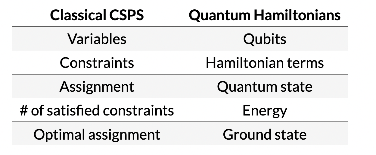
CS view of Hamiltonians: Hamiltonians are quantum analogues of constraint satisfaction problems (CSPs).
Constraint Satisfaction Problems
An instance of a $k$-local CSP consists of:
- variables $x_1,\ldots,x_n$ that can take boolean values
- constraints $C_1,\ldots,C_m$ where each $C_j$ indicates the allowed values for a subset $S_j$ of variables.
Example: 3SAT is a $3$-local CSP where each of the constraints $C_j$ are of the form
$$ C_j = x_1 \vee x_5 \vee \neg x_7 $$Constraint Satisfaction Problems
The important questions: given a CSP,
- Is it satisfiable?
- What is the maximum number of constraints that can be simultaneously satisfied?
These questions generally correspond to NP-complete problems.
Max-Cut Problem
Given a graph $G = (V,E)$, find a partition of vertices that maximizes number of cut edges.
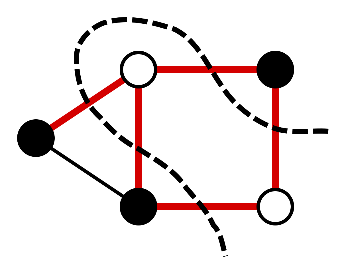
Equivalently, a $2$-local CSP:
- For every vertex $v \in V$, a variable $x_v$.
- For every edge $e = (u,v) \in E$, a constraint $x_u \neq x_v$.
Max-Cut Problem
NP-hard to find the optimal cut.
However, it is possible to find an approximately optimal cut in polynomial time. The Goemans-Williamson algorithm can find a cut that achieves $87.8\%$ of the maximum possible.
Open question: is there a polynomial-time algorithm that achieves a better approximation of Max-Cut?
Classical-Quantum Dictionary
Hamiltonians
Mathematically, a $n$-qubit Hamiltonian $H$ is a Hermitian $n$-qubit matrix. It has dimension $2^n \times 2^n$.
By the spectral theorem, we can diagonalize $H = \sum_j E_j \, \ketbra{v_j}{v_j}.$
$\{ E_j \}_j$ are the energy levels of $H$. The vector $\ket{v_j}$ is an energy eigenstate with energy $E_j$.
Hamiltonians
The physical interpretation of a Hamiltonian $H$: it assigns an average energy to every $n$-qubit state $\ket{\psi}$. Energy of $\ket{\psi}$ with respect to $H$: $\bra{\psi} H \ket{\psi}$
Since energy eigenstates form a basis, we can write $\ket{\psi} = \sum_j \alpha_j \ket{v_j}$.
Thus energy of $\ket{\psi} = \bra{\psi} \Big( \sum_j E_j \ketbra{v_j}{v_j} \Big) \ket{\psi}$
$ \quad = \sum_j E_j \, |\langle \psi \mid v_j \rangle |^2 = \sum_j E_j |\alpha_j|^2$.
Hamiltonians
The states $\ket{\psi}$ with minimum energy with respect to $H$ are called ground states. The minimum energy is called ground energy.
$E_{ground} = \min_{\ket{\psi}} \bra{\psi} H \ket{\psi}$.
Exercise: The ground energy of $H$ is equal to the minimum eigenvalue of $H$, and all ground states are eigenvectors of $H$.
Local Hamiltonians
Physics focuses on local Hamiltonians, which means
$$ H = H_1 + H_2 + \cdots + H_m $$where each $H_j$ is a local Hamiltonian term, acting nontrivially on a small set of qubits.
Just like how quantum circuits consist of local gates acting on one or two qubits at a time, the interesting Hamiltonians in physics are built out of local terms.
Local Hamiltonians
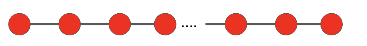
Example: a line of interacting particles.
Each vertex corresponds to a qubit. Qubits only interact with neighboring qubits.
For every pair of neighbors $(j,j+1)$, there is a Hamiltonian term
$$ H_{j,j+1} = I_{j-1} \otimes h_{j,j+1} \otimes I_{n-{j-1}} $$where $h_{j,j+1}$ is a $4 \times 4$ Hermitian matrix.
Local Hamiltonians
Example: a line of interacting particles.
The overall Hamiltonian is
$$ H = \sum_{j} H_{j,j+1} $$Note that $H$ is a gigantic matrix ($2^n \times 2^n$), but it is built out of a small number of local matrices $h_{j,j+1}$. Just like how an $n$-qubit quantum unitary can be built out of a small number of local unitary gates.
Local Hamiltonians
Local Hamiltonians are prevalent in physics because the laws of nature are inherently local: particles interact with nearby ones.
Depending on what kind of physical phenomena is being investigated, physicists will write down different local Hamiltonians.
For example, electric field, magnetic field, nuclear forces, etc...
Ising Hamiltonian
An important model of magnetism in physics.
Each particle is a magnet that points up ($\ket{0}$) or points down ($\ket{1}$). Neighboring magnets want to anti-align.
There is also a global magnetic field that encourages all magnets to point in a specific direction.
Ising Hamiltonian
Recall $Z = \begin{pmatrix} 1 & 0 \\ 0 & -1 \end{pmatrix}$.
The 1D Ising Model is
$$ H = - \sum_{i=1}^{n-1} Z_i \otimes Z_{i+1} + \mu \sum_{i=1}^n Z_i $$where $\mu$ = magnetic field strength parameter.
Note: $Z_i \otimes Z_{i+1}$ and $Z_i$ are implicitly tensored with identity operators on all the other qubits. Each term is a $2^n \times 2^n$ matrix!
Why does $\mu Z_i$ capture the "global magnetic field" on the $i$'th qubit?
We can diagonalize $Z = \ketbra{0}{0} - \ketbra{1}{1} = \begin{pmatrix} 1 & 0 \\ 0 & 0 \end{pmatrix} - \begin{pmatrix} 0 & 0 \\ 0 & 1 \end{pmatrix}$.
Thus $\mu Z_i$ has energy $\mu$ for any state where $i$'th qubit is in state $\ket{0}$, and $-\mu$ where $i$'th qubit is in state $\ket{1}$.
If $\mu > 0$, then $i$'th qubit "prefers" to be in state $\ket{1}$ (because that's lower energy); otherwise it prefers $\ket{0}$.
Why does $Z_i \otimes Z_{i+1}$ capture the "anti-alignment" interaction between qubits $i$ and $i+1$?
Its spectral decomposition:
$Z_i \otimes Z_j = \Big (\ketbra{0}{0}_i - \ketbra{1}{1}_i \Big ) \otimes \Big (\ketbra{0}{0}_{i+1} - \ketbra{1}{1}_{i+1} \Big) $
$ \qquad = \ketbra{00}{00}_{i,i+1} + \ketbra{11}{11}_{i,i+1} - \ketbra{01}{01}_{i,i+1} - \ketbra{10}{10}_{i,i+1}$
The lower energy configurations are where qubits $i$ and $i+1$ point in opposite directions!
Ising Hamiltonian
The energy of a state $\ket{\psi}$ in the Ising model is
$$ \bra{\psi} H \ket{\psi} = \sum_{i=1}^{n-1} \bra{\psi} Z_i \otimes Z_{i+1} \ket{\psi} + \mu \sum_{i=1}^n \bra{\psi} Z_i \ket{\psi} $$The "anti-alignment" and "global magnetic field" terms compete with each other!
Exercise: what are the minimum energy configurations, depending on $\mu$?
The Ising Hamiltonian is a classical Hamiltonian, because it is diagonal in the standard basis. In particular, ground states are all classical basis states.
An example of a quantum Hamiltonian is the Transverse Field Ising Model:
$$ H = -\sum_{i=1}^{n-1} Z_i \otimes Z_{i+1} + g \sum_{i=1}^n X_i $$where $X = \begin{pmatrix} 0 & 1 \\ 0 & 1 \end{pmatrix}$.
The ground states of this Hamiltonian are generally entangled and non-classical.
The important questions: given a (local) Hamiltonian $H$,
- What is its ground energy?
- What are its ground states?
- How does a quantum system, governed by $H$, evolve over time?
Ground states
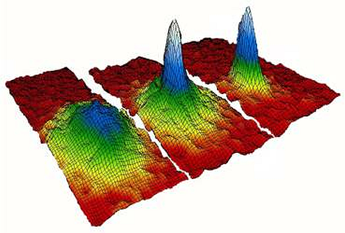
Ground states are interesting because they represent quantum systems at low temperatures (e.g. near absolute zero). Ground states of quantum Hamiltonians tend to exhibit bizarre quantum effects.

Ground states
Computing ground states and ground energies of Hamiltonians is not easy!
In fact, it is generally an NP-hard problem.
Finding ground states of local Hamiltonians is analogous to finding optimal solutions of CSPs.
Next time
Time evolution under a Hamiltonian, and simulating it.