Admin
- Pset2 due Sunday, October 9, 11:59pm.
- Henry, please record the lecture!
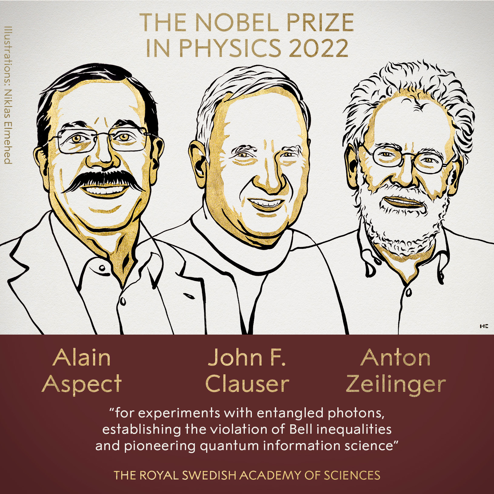
John Clauser
Alain Aspect
Anton Zeilinger
Last Time
- Simons Algorithm
Quantum Fourier Transformation
Quantum algorithm that implements the Discrete Fourier Transform (DFT) on exponentially large dimension.
It is the heart of many powerful quantum algorithms such as
- Shor's factoring algorithm
- Phase estimation algorithm
- Algorithms for solving hidden subgroup problem
Discrete Fourier Transformation
A method to uncover hidden, periodic structure in vectors. Used everywhere in engineering, science, and mathematics.
An example of a vector that represents a noisy signal whose characteristics we'd like to analyze.
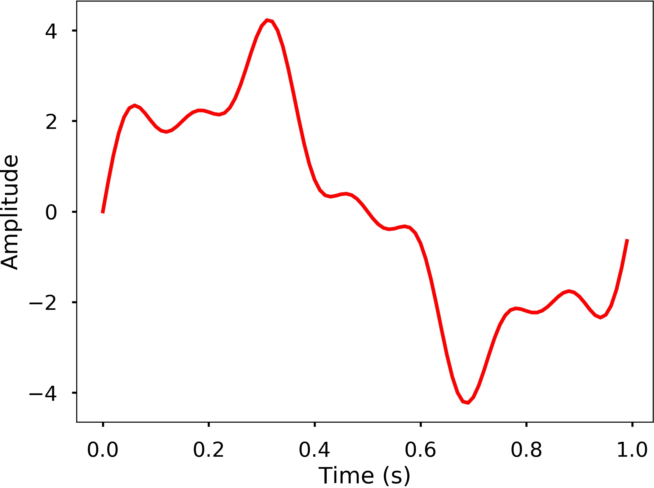
The entries of the vector correspond to equally spaced time points and the value of the entry corresponds to the signal amplitude at that time.
Discrete Fourier Transformation
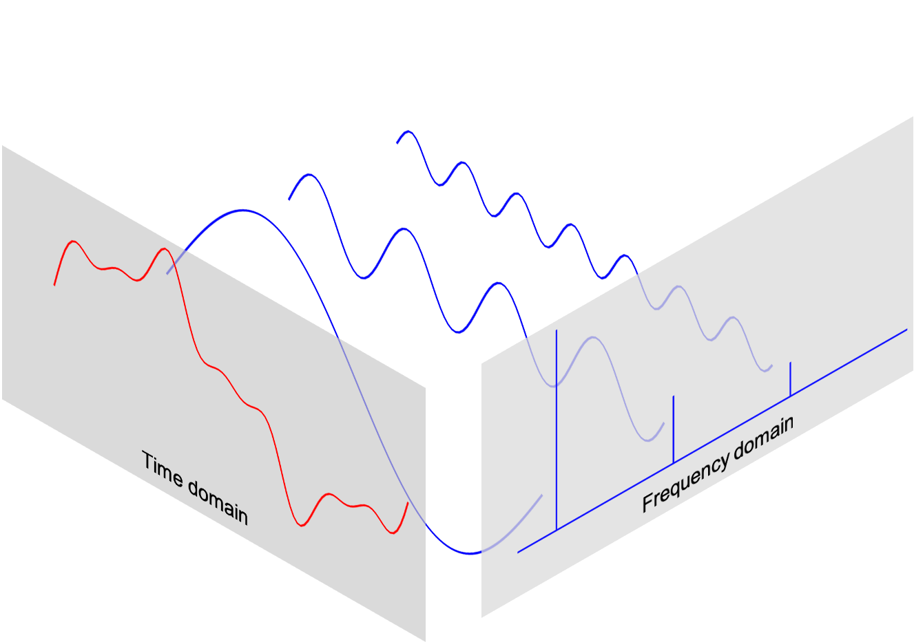
The Discrete Fourier Transform (DFT) is a method to express every vector (i.e. every signal) as a linear combination of simple periodic vectors (i.e. complex sinusoidal signals).
Visually:
Discrete Fourier Transformation
The Discrete Fourier Transform (DFT) is a method to express every vector (i.e. every signal) as a linear combination of simple periodic vectors (i.e. complex sinusoidal signals).
Mathematically: every vector $\ket{\psi} \in \C^N$ can be written as $$ \ket{\psi} = \sum_{j = 0}^{N-1} \hat{\psi}_j \, \ket{f_j} $$ where $\{ \ket{f_0}, \ket{f_1}, \ldots, \ket{f_{N-1}} \}$ is the $\mathbb{Z}_N$-Fourier basis.
The Fourier basis
 The Fourier basis vectors are
$$
\ket{f_j} = \frac{1}{\sqrt{N}} \sum_{k=0}^{N-1} \omega_N^{j k} \, \ket{k}
$$
for $j = 0, 1, \ldots, N-1$ where
$$
\omega_N = \exp \Big( 2\pi i/N \Big)
$$
are the $N$'th roots of unity.
The Fourier basis vectors are
$$
\ket{f_j} = \frac{1}{\sqrt{N}} \sum_{k=0}^{N-1} \omega_N^{j k} \, \ket{k}
$$
for $j = 0, 1, \ldots, N-1$ where
$$
\omega_N = \exp \Big( 2\pi i/N \Big)
$$
are the $N$'th roots of unity.
Exercise: These vectors are orthonormal.
The Fourier basis
Example: $N = 8, j = 0$.
$$ \ket{f_0} = \frac{1}{\sqrt{N}} \sum_{k = 0}^{N-1} \ket{k} = \frac{1}{\sqrt{N}} \Big( 1, 1, \ldots, 1 \Big)^\top $$Visually: 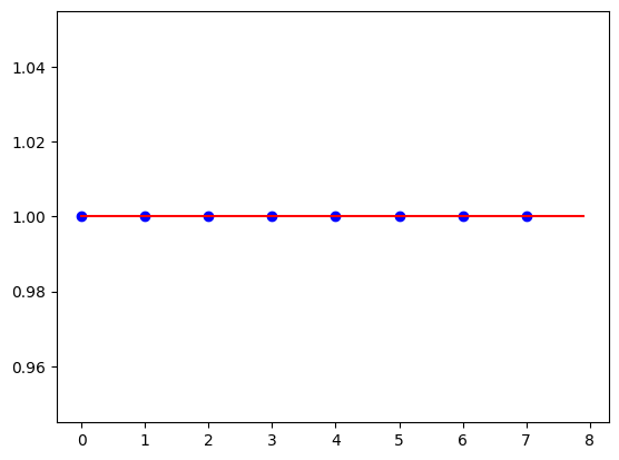
The Fourier basis
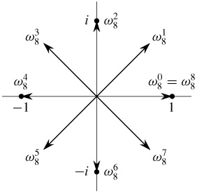
Example: $N = 8, j = 1$.
$$ \ket{f_1} = \frac{1}{\sqrt{N}} \sum_{k=0}^{N-1} \omega_N^k \ket{k} = \frac{1}{\sqrt{N}} \Big( 1,\omega_8, \omega^2_8, \ldots, \omega^7_8 \Big)^\top $$Visually, the real component of $\omega_N^{jk}$: 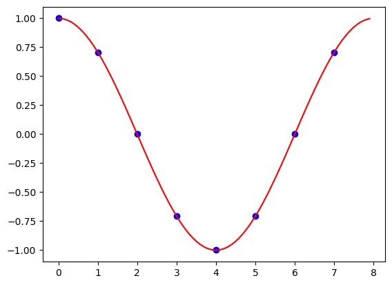
The Fourier basis
Example: $N = 8, j = 5$.
$$ \ket{f_5} = \frac{1}{\sqrt{N}} \sum_{k=0}^{N-1} \omega_N^{5k} \ket{k} = \frac{1}{\sqrt{N}} \Big( 1,\omega_8^5, \omega^2_8, \omega^7_8, \ldots \Big)^\top $$Visually, the real component of $\omega_N^{jk}$: 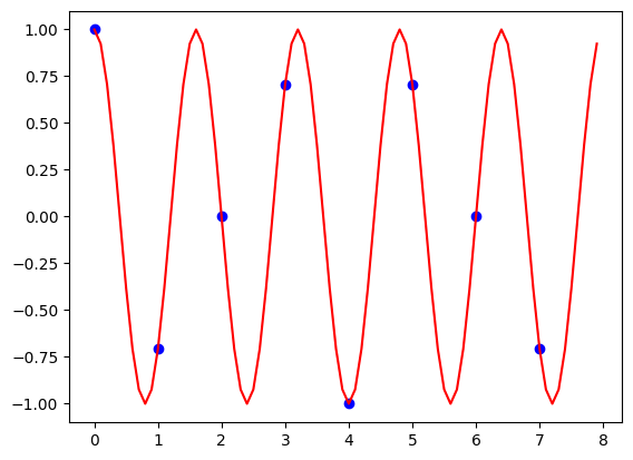
Let $\ket{\psi} = \sum_{j=0}^{N-1} \psi_j \ket{j}$ be a signal represented in the standard basis.
In the Fourier basis, $\ket{\psi}$ can be written as $\ket{\psi} = \sum_{j = 0}^{N-1} \hat{\psi}_j \, \ket{f_j}$ for some Fourier coefficients $\hat{\psi}_j$.
The magnitude $|\hat{\psi}_j|^2$ of the $j$'th Fourier coefficient quantifies the contribution of $\ket{f_j}$ to $\ket{\psi}$.
What's the relationship between the amplitudes $\{ \psi_0,\psi_1,\ldots,\psi_{N-1}\}$ and the Fourier coefficients $\{ \hat{\psi}_0, \hat{\psi}_1,\ldots,\hat{\psi}_{N-1} \}$?
They are related by a unitary transformation $F_N$ (which is the DFT). It maps $\ket{f_j} \mapsto \ket{j}$.
Applying $F_N$ to $\ket{\psi}$ yields the vector
$$ F_N \ket{\psi} = \ket{\hat{\psi}} = \sum_{j=0}^{N-1} \hat{\psi}_j \ket{j}. $$The Fourier coefficients of $\ket{\psi}$ have been turned into amplitudes in the standard basis of $\ket{\hat{\psi}}$.
Quantum Fourier Transform
Let $N = 2^n$. The Quantum Fourier Transform (QFT) is a quantum algorithm for implementing the $n$-qubit unitary $F_N$ while taking only $\mathrm{poly}(n)$ time.
QFT maps quantum states $\ket{\psi}$ to their Fourier transform state $\ket{\hat{\psi}} = \sum_j \hat{\psi}_j \ket{j}$.
Here, we associate $\ket{j}$ with the $n$-qubit state $\ket{j_1 j_2 \cdots j_n}$, the binary representation of $j$.
Quantum Fourier Transform
The best classical algorithm for computing DFT of a $N$-dimensional vector is called the Fast Fourier Transform (FFT), which takes $O(N \log N)$ time.
Does this constitute an exponential speedup?
Quantum Fourier Transform
Not exactly. The Fast Fourier Transform gets an input that is a classical $N$-dimensional vector $\ket{\psi}$, and outputs another $N$-dimensional vector $\ket{\hat{\psi}}$.
On the other hand, QFT gets an input vector in quantum form, and produces an output vector in quantum form.
The Fourier coefficients $\{\hat{\psi}_j\}_j$ are not readily accessible: measuring $\ket{\hat{\psi}}$ produces basis vector $\ket{j}$ with probability $|\hat{\psi}_j|^2$, but afterwards all other information about the Fourier coefficients is lost.
The Fourier transform unitary $F_2$
Example: $N = 2$ (single-qubit unitary)
$$ F_2 = \frac{1}{\sqrt{2}} \begin{pmatrix} 1 & 1 \\ 1 & -1 \end{pmatrix}~. $$We've seen this before...
The Fourier transform unitary $F_4$
Example: $N = 4$ (two qubits)
$$ F_4 = \frac{1}{\sqrt{4}} \begin{pmatrix} 1 & 1 & 1 & 1 \\ 1 & i & -1 & -i \\ 1 & -1 & 1 & -1 \\ 1 & -i & -1 & i \end{pmatrix}~. $$The rows/columns are ordered by $\ket{0}, \ket{1}, \ket{2}, \ket{3}$, which in binary are $\ket{00}, \ket{01}, \ket{10}, \ket{11}$.
The Fourier transform unitary $F_4$
Example: $N = 4$ (two qubits). Reordering the rows/columns according to $\ket{00}$, $\ket{10}, \ket{01}$, $\ket{11}$.
$$ F_4 = \frac{1}{\sqrt{4}} \begin{pmatrix} 1 & 1 & 1 & 1 \\ 1 & -1 & i & -i\\ 1 & 1 & -1 & -1 \\ 1 & -1 & -i & i \end{pmatrix}~. $$Can you spot recursive structure?
The Fourier transform unitary $F_4$
Example: $N = 4$ (two qubits). Reordering the rows/columns according to $\ket{00}$, $\ket{10}, \ket{01}$, $\ket{11}$.
$$ F_4 = \frac{1}{\sqrt{4}} \begin{pmatrix} 1 & 1 & 1 & 1 \\ 1 & -1 & i & -i\\ 1 & 1 & -1 & -1 \\ 1 & -1 & -i & i \end{pmatrix} = \frac{1}{\sqrt{2}} \begin{pmatrix} F_2 & A_2 F_2 \\ F_2 & -A_2 F_2 \end{pmatrix} $$where
$$ A_2 = \begin{pmatrix} 1 & 0 \\ 0 & i \end{pmatrix} $$The Fourier transform unitary $F_N$
For general $N = 2^n$, if we order the columns where all the "even" columns are on the left, and all the "odd" columns are on the right, then $$ F_N = \frac{1}{\sqrt{2}} \begin{pmatrix} F_{\frac{N}{2}} & A_{\frac{N}{2}} F_{\frac{N}{2}} \\ F_{\frac{N}{2}} & -A_{\frac{N}{2}} F_{\frac{N}{2}} \end{pmatrix} $$ where $$ A_{N/2} = \begin{pmatrix} 1 & & & & \\ & \omega_N & & & \\ & & \omega_N^2 & &\\ & & & \ddots & \\ & & & & \omega_N^{N/2-1} \end{pmatrix} $$
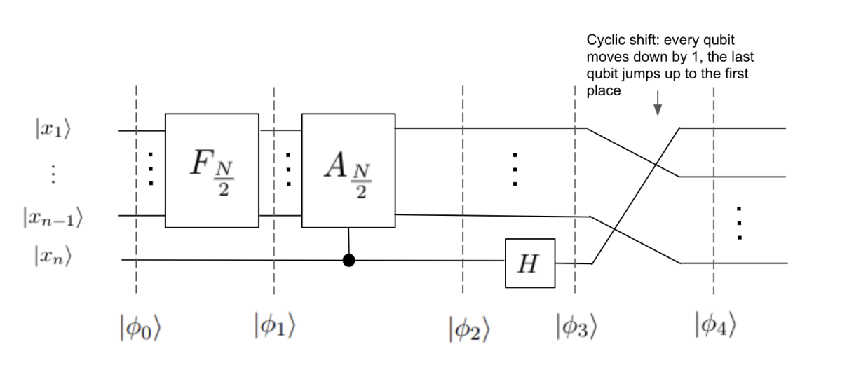
The Quantum Fourier Transform circuit
The recursive formula for $F_N$ inspires a recursive construction for the QFT circuit. Assume we already have circuits for the unitaries $F_{N/2}$ and $A_{N/2}$. Then the the circuit for $F_N$ looks like
The phase circuit $A_{N/2}$
How is the circuit for $A_{N/2}$ implemented?
Note that the unitary acts on $n-1$ qubits, and for all $y \in \{0,1\}^{n-1}$ the unitary maps
$$ \ket{y_1,\ldots,y_{n-1}} \mapsto \omega_N^{\mathrm{toint}(y)} \ket{y_1,\ldots,y_{n-1}} $$where $$ \mathrm{toint}(y) = y_1 2^{n-2} + y_2 2^{n-3} + \cdots + y_{n-1} $$
The phase circuit $A_{N/2}$
Expanding and regrouping we get \begin{align*} \ket{y_1,\ldots,y_{n-1}} &\mapsto \omega_N^{2^{n-2} \cdot y_1} \omega_N^{2^{n-3} \cdot y_2} \cdots \omega_N^{y_{n-1}} \ket{y_1,\ldots,y_{n-1}} \\ &= \Big( \omega_N^{2^{n-2} \cdot y_1} \ket{y_1} \Big) \Big( \omega_N^{2^{n-3} \cdot y_2} \ket{y_2} \Big) \cdots \Big( \omega_N^{y_{n-1}} \ket{y_{n-1}} \Big) \end{align*}
The phase circuit $A_{N/2}$
It is just a tensor product unitary!
$$ A_{N/2} = P(1/4) \otimes P(1/8) \otimes \cdots \otimes P(1/2^n) $$where $$ P(\varphi) = \begin{pmatrix} 1 & 0 \\ 0 & e^{2\pi i \varphi} \end{pmatrix} $$
The Quantum Fourier Transform circuit
Complexity analysis. Let $T(n)$ denote the number of gates used to construct $F_N$. It satisfies $T(n) = T(n-1) + O(n)$. Unrolling the recursion, we get $T(n) = O(n^2)$.
Analysis of the Quantum Fourier Transform circuit
Why does it work?
It's a couple pages of algebra... take a look at the scribe notes if you're interested!
Application of QFT: Phase Estimation
Phase Estimation Algorithm (PEA) is one of the most important subroutines in quantum computing.
Linear algebra fact: the eigenvalues of unitary matrices are all complex numbers of the form $e^{2\pi i \theta}$.
Goal of PEA: Given blackbox access to an unknown unitary $U$, and a quantum state $\ket{\psi}$ that is an eigenvector of $U$ (also called an eigenstate) with eigenvalue $e^{2 \pi i \theta}$, estimate $\theta$.
Phase Estimation Algorithm
Assume for simplicity that $\theta$ can be represented using exactly $t$ bits. In other words the binary representation of $\theta$ looks like $$ \theta = 0.\theta_1 \theta_2 \cdots \theta_t $$ where $\theta_1,\theta_2,\ldots \in \{0,1\}$. This is equivalent to $$ \theta = \frac{\theta_1}{2} + \frac{\theta_2}{2^2} + \cdots + \frac{\theta_t}{2^t}. $$
Phase Estimation Algorithm
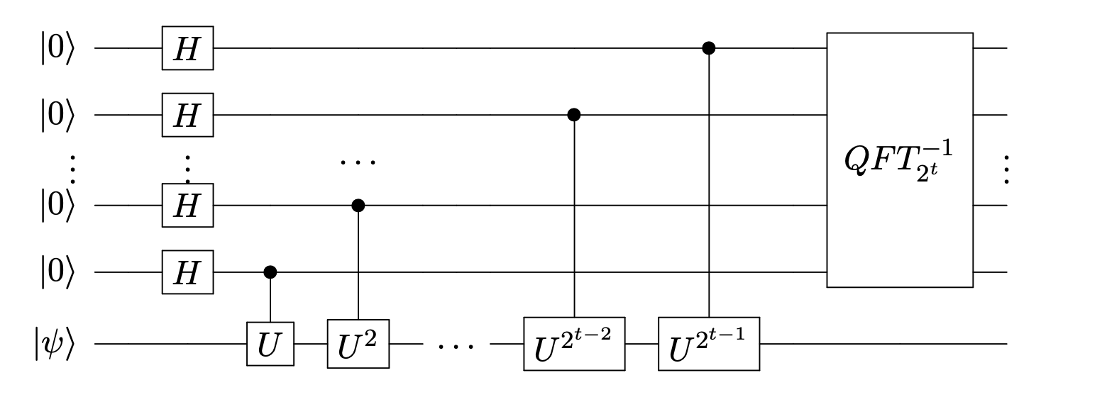
Measuring the first $t$ qubits will yield $\ket{\theta_1,\theta_2,\ldots,\theta_t}$.
Next time
We'll analyze the Phase Estimation algorithm, and see applications of it.