Last Time: classical reversible computing
$d$-dimensional systems:
- State labels: $\ket{0},\ldots,\ket{d-1}$.
- Transformations $T$: permutations on $d$ labels
Composite systems using tensor product:
- If system $A$ in state $\ket{x}$, system $B$ in state $\ket{y}$,
then joint state is $\ket{x} \otimes \ket{y}$.
Can implement universal classical computation.
Last Time: classical reversible computing, linear algebra-ized
States represented as column vectors: $$ |0\rangle = \begin{pmatrix} 1 \\ 0 \\ \vdots \end{pmatrix} \quad |1\rangle = \begin{pmatrix} 0 \\ 1 \\ \vdots \end{pmatrix} \qquad \cdots\qquad \ket{d-1} = \begin{pmatrix} \vdots \\ 0 \\ 1 \end{pmatrix} $$
Transformations are $d \times d$ permutation matrices, e.g., $$ T = \begin{pmatrix} 0 & 1 & 0 & 0 \\ 0 & 0 & 1 & 0 \\ 0 & 0 & 0 & 1 \\ 1 & 0 & 0 & 0 \end{pmatrix} $$
Updating a state $\ket{x}$ by transformation $T$ is matrix-vector multiplication $T \ket{x}$.
Tensor product of vectors and matrices corresponds to combining states and transformations
Making the quantum leap
A bit is a classical system with two distinguishable states $\ket{0}, \ket{1}$, also called Classical states, or standard basis states.
A **qubit** (quantum bit) can be in a **superposition** of the classical states $\ket{0},\ket{1}$.
Mathematically, states of a qubit are **complex linear combination** of $\ket{0},\ket{1}$:
$$ \ket{\psi} = \alpha \ket{0} + \beta \ket{1} \\ = \alpha \begin{pmatrix} 1 \\ 0 \end{pmatrix} + \beta \begin{pmatrix} 0 \\ 1 \end{pmatrix} \\ = \begin{pmatrix} \alpha \\ \beta \end{pmatrix}. $$where $\alpha,\beta \in \mathbb{C}$ are complex numbers satisfying $|\alpha|^2 + |\beta|^2 = 1$.
In other words, $\ket{\psi}$ is a two-dimensional unit vector in $\mathbb{C}^2$.
Example: a qubit can be in the state
$$ \frac{1}{\sqrt{2}} \ket{0} + \frac{1}{\sqrt{2}} \ket{1}. $$Another example:
$$ \frac{1}{\sqrt{2}} \ket{0} - \frac{i}{\sqrt{2}} \ket{1} = \frac{1}{\sqrt{2}} \begin{pmatrix} 1 \\ -i \end{pmatrix}. $$A non-valid qubit state:
$$ i \ket{0} - \frac{1}{2} \ket{1}. $$So... what is a qubit?
A qubit in the state $\alpha \ket{0} + \beta \ket{1}$ is commonly said to be $\ket{0}$ and $\ket{1}$ "at the same time". But what does that mean?
$\alpha, \beta$ are like probabilities, except they can be negative or even complex numbers!
$\alpha,\beta$ are called the **amplitudes** of the states $\ket{0}$ and $\ket{1}$, respectively.
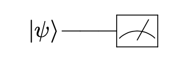
Observing qubits
The state of a qubit cannot be directly observed. It must be **measured**, yielding a classical state $\ket{0}$ or $\ket{1}$ with probabilities
Because qubit states have unit length, these probabilities add up to $1$.
This formula is called the **Born Rule**.
Observing qubits
After measurement, the system becomes **classical.**
The state of qubit **collapses** to either $\ket{0}$ or $\ket{1}$, and the previous state is lost.
**In quantum mechanics, measurement generally disturbs the system.**
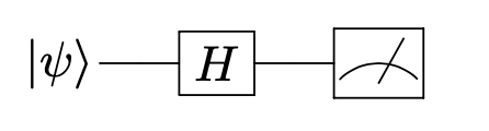
We represent qubit measurements using this diagram:
Observing qubits
If the state collapses to the classical state $\ket{0}$ and we measure it again, it stays in state $\ket{0}$ with probability $1$. Same with collapsing to $\ket{1}$.
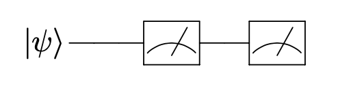 =
=
**Measuring a system twice is the same as measuring once.**
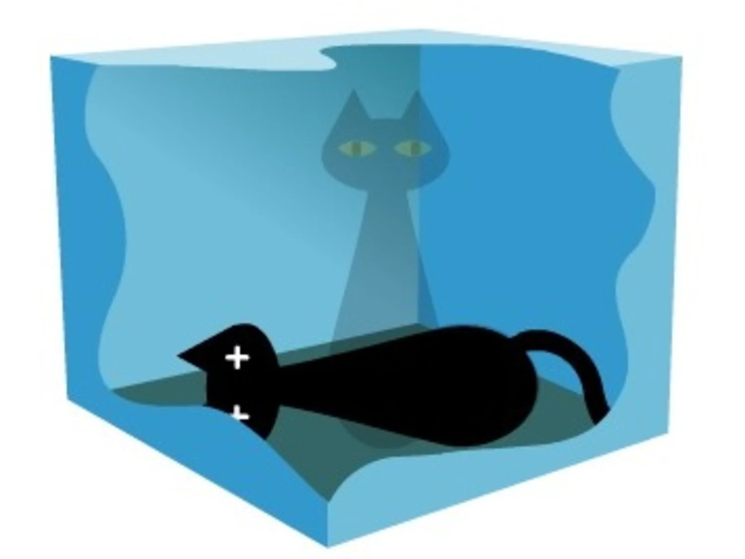
Example: Schrödinger's cat.
A box with two classical states:
$$ \text{sleeping cat: } \ket{0} \qquad \qquad \text{awake cat: } \ket{1} $$In quantum mechanics, the box can be in a superposition of
sleeping and awake cat,
as long as you don't open the box (i.e. measure it).
Example: Schrödinger's cat.
Suppose the box starts in the state $\frac{1}{\sqrt{3}} \ket{0} - i \, \frac{\sqrt{2}}{\sqrt{3}} \ket{1}$ and is measured.
With probability $\Big | \frac{1}{\sqrt{3}} \Big |^2 = \frac{1}{3}$, the state collapses to $\ket{0}$ (i.e., sleeping cat).
With probability $\Big | - i \frac{\sqrt{2}}{\sqrt{3}} \Big |^2 = \frac{2}{3}$, the state collapses to $\ket{1}$ (i.e., awake cat).
Doesn't this contradict Landauer's principle?
Transformations on qubits
In addition to measurement, the state of a qubit can change via a **unitary transformation**. Just like transformations in classical reversible computing, unitary tranformations can be represented as matrices.
We represent a unitary transform $U$ acting on state $\ket{\psi}$ using the following circuit diagram:
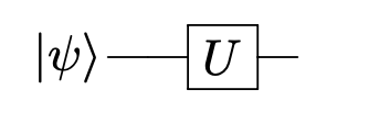
Several equivalent definitions of $d \times d$ unitary matrices $U$:
Definition 1. The inverse of $U$ is its Hermitian conjugate $U^\dagger$, pronounced "$U$ dagger", whose $(i,j)$'th entry is the complex conjugate of the $(j,i)$'th entry of $U$.
$$ U^\dagger_{i,j} = \overline{U}_{j,i} $$Definition 2. $U$ maps unit vectors to unit vectors (i.e. quantum states to quantum states)
Definition 3. The rows of $U$ form an orthonormal basis for $\mathbb{C}^d$, and the columns form an orthonormal basis for $\mathbb{C}^d$.
Definition 4. $U$ preserves the inner products between vectors: inner product between $\ket{\psi}$ and $\ket{\theta}$ is the same as the inner product between $U\ket{\psi}$ and $U\ket{\theta}$.
Examples of qubit unitary matrices
Identity matrix $I = \begin{pmatrix} 1 & 0 \\ 0 & 1 \end{pmatrix}$
For all qubit states $\ket{\psi}$, $I \ket{\psi} = \ket{\psi}$.
Examples of qubit unitary matrices
Bit flip matrix $X = \begin{pmatrix} 0 & 1 \\ 1 & 0 \end{pmatrix}$
So far, have only seen classical transformations.
Examples of qubit unitary matrices
Phase flip matrix $Z = \begin{pmatrix} 1 & 0 \\ 0 & -1 \end{pmatrix}$
Examples of qubit unitary matrices
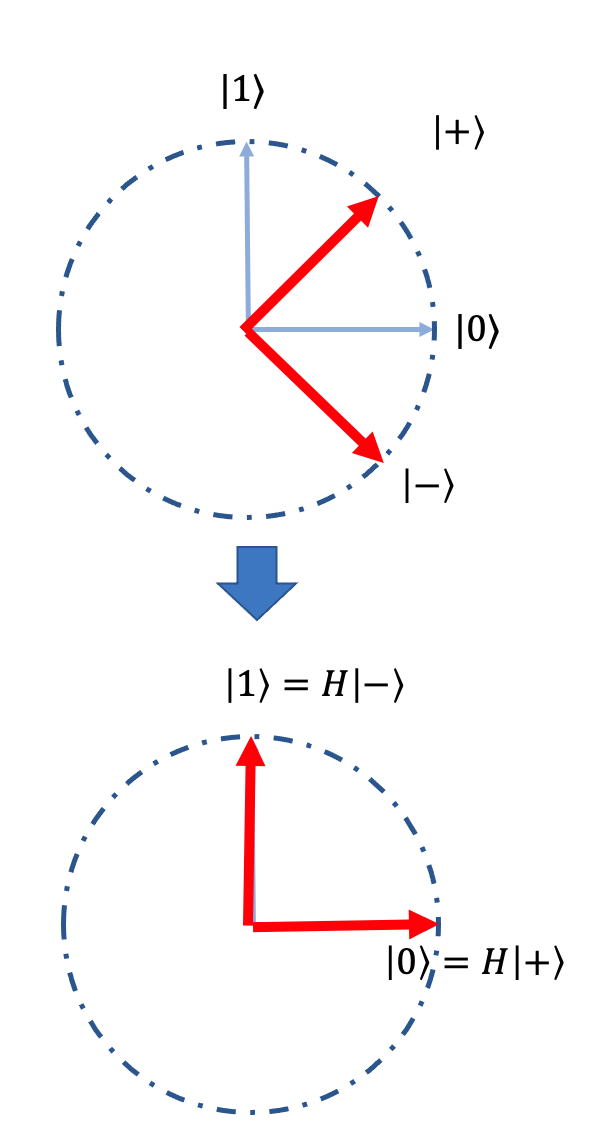
Hadamard matrix $H = \frac{1}{\sqrt{2}} \begin{pmatrix} 1 & 1 \\ 1 & -1 \end{pmatrix}$
$$ H \ket{0} = \cdots \text{(do on board)} \cdots $$$$ H \ket{1} = \cdots \text{(do on board)} \cdots $$$H$ maps classical basis states $\ket{0},\ket{1}$ into quantum superpositions.
Quantum vs classical bits
What is the difference between
$\ket{+} = \frac{1}{\sqrt{2}} \Big ( \ket{0} + \ket{1} \Big)$ and
$\ket{-} = \frac{1}{\sqrt{2}} \Big ( \ket{0} - \ket{1} \Big)$?
Measuring both states yields the same statistical outcomes: $\ket{0},\ket{1}$ with 50% probability each!
Quantum vs classical bits
Suppose we were physically handed a qubit (say Schödinger's box) whose state $\ket{\psi}$ was either $\ket{+}$ or $\ket{-}$. Is there a way we can tell the difference?
Opening the box (i.e., measuring) would yield a sleeping or awake cat with equal probability in both cases.
Case 1: $\ket{\psi} = \ket{+}$. Applying $H$, we get
$$ H \ket{+} = \cdots \text{(show on the board)} \cdots = \ket{0} $$Measuring yields $\ket{0}$ all the time!
Quantum vs classical bits
Solution: Apply $H$ to qubit before measuring!
Case 2: $\ket{\psi} = \ket{-}$. Applying $H$, we get
$$ H \ket{-} = \cdots \text{(show on the board)} \cdots = \ket{1} $$Measuring yields $\ket{1}$ all the time!
Quantum vs classical bits
The states $\ket{+} = \frac{1}{\sqrt{2}} \begin{pmatrix} 1 \\ 1 \end{pmatrix}$ and $\ket{-} = \frac{1}{\sqrt{2}} \begin{pmatrix} 1 \\ -1 \end{pmatrix}$ form an orthonormal basis for $\mathbb{C}^2$.
In quantum mechanics, orthogonal states can be **perfectly distinguished** by applying an appropriate unitary matrix and then measuring in the standard basis.
The Hadamard matrix maps the $\big \{ \ket{+}, \ket{-} \big \}$ basis to the standard $\big \{ \ket{0}, \ket{1} \big \}$ basis (and vice versa).
Quantum vs classical bits
**Takeway**: Minus signs in the amplitudes matter!
More precisely, **relative phases** between the classical basis states matter.
On the other hand, **global phases** don't matter.
There is no quantum process (unitary + measurement) to distinguish between $\ket{\psi}$ and $-\ket{\psi}$, or in fact $\alpha \ket{\psi}$ for any complex phase $\alpha = e^{i \theta}$. Can you see why?
Quantum vs classical bits, take 2
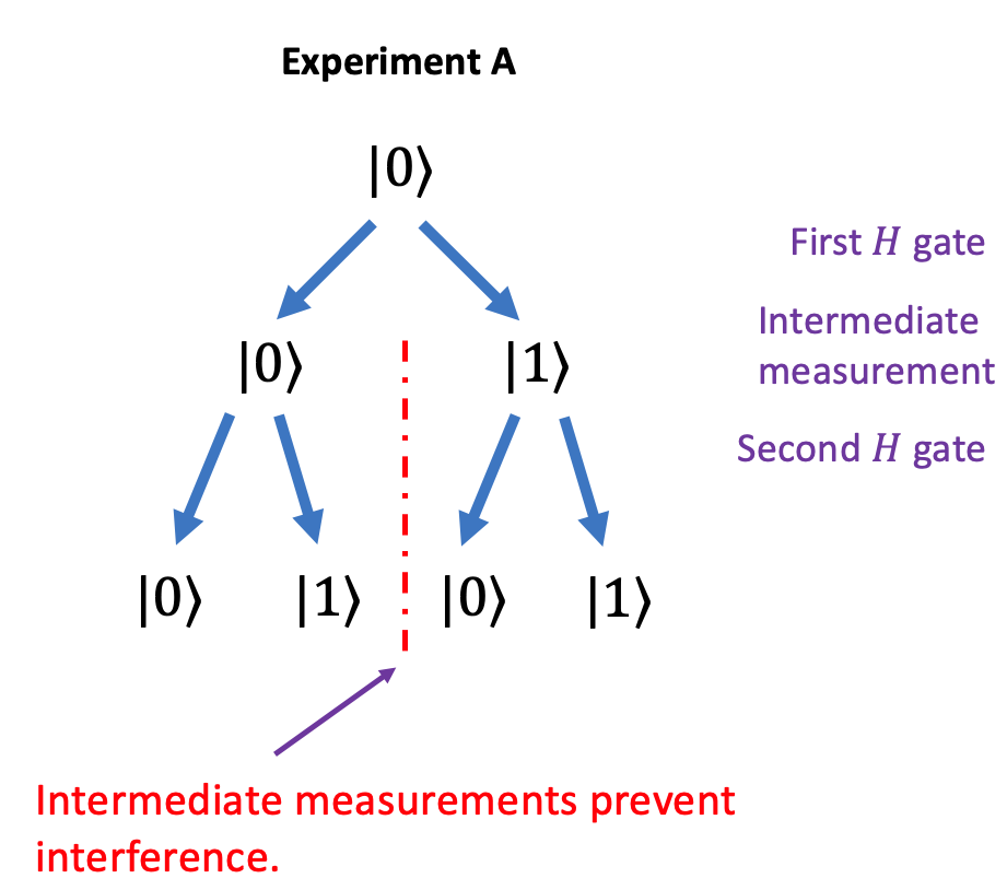
Consider the following quantum circuit, called Experiment A:
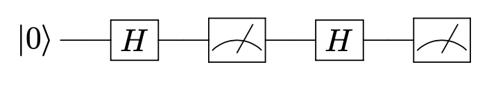
Final distribution of outcomes: $\ket{0},\ket{1}$ with equal probability.
Based on this, one might conclude that the Hadamard gate simply creates a random classical bit!
Quantum vs classical bits, take 2
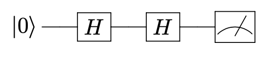
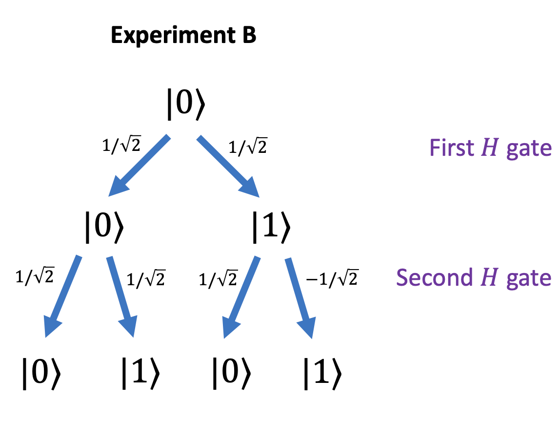
Now consider Experiment B, where we only measure the system at the end:
Quantum vs classical bits, take 2
Now consider Experiment B, where we only measure the system at the end:
Final distribution of outcomes: $\ket{0}$ always.
**Inserting or removing intermediate measurement can drastically change the behavior of a quantum system!**
Quantum interference
Applying multiple unitary operations to a qubit gives rise to a tree of “paths” between states.
An edge between state $\ket{a}$ to $\ket{b}$ has a transition amplitude associated with, depending on the unitary.
Quantum interference
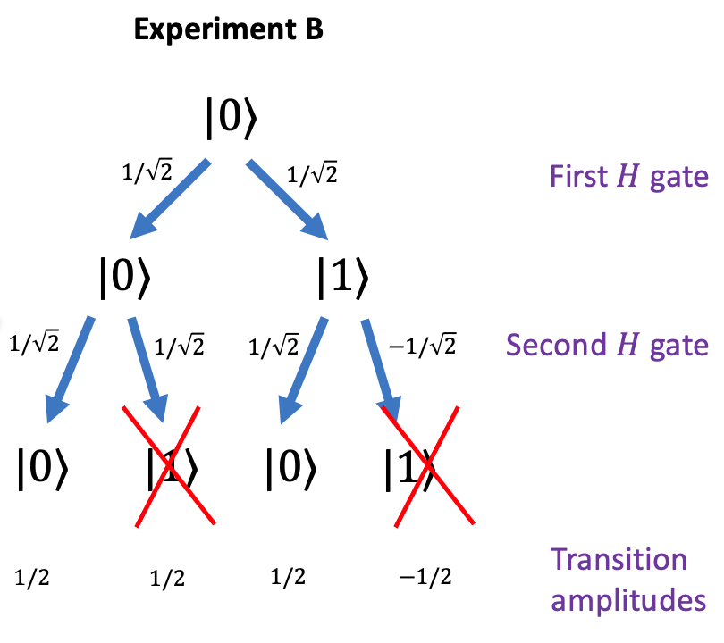
Each path has associated transition amplitude: product of amplitudes along the path.
Before measurement, amplitude of ending up in state $\ket{b}$ is the sum of transition amplitudes of all paths that end at $\ket{b}$.
Since transition amplitudes can be positive, negative, or even complex, the paths leading to $\ket{b}$ can constructively or destructively interfere with each other!
Quantum interference
If there is an intermediate measurement, only paths consistent with the measurement outcome are added up.
**Takeway**: Intermediate measurements destroy superpositions and prevent interference!
In classical physics, we only add up probabilities, which are positive. In quantum physics, we add up amplitudes, which can be negative. Interference is an example of "quantum weirdness".
Summary of one qubit
- A qubit state $\ket{\psi}$ is a two-dimensional unit vector
- Measuring qubits yields $\ket{0},\ket{1}$ with probabilities determined by the Born rule.
- State of qubit can also change via unitary matrices.
- Positive and negative transition amplitudes lead to interference.
- Measurements disrupt interference.
Dirac Notation
The $\ket{\psi}$ notation is called **Dirac notation**, after the quantum physicist Paul Dirac.
Mathematically, $\ket{\psi}$ ("ket vector") is a column vector.
The dual/Hermitian conjugate of column vectors (i.e., row vectors) are called "bra vectors":
$$ \bra{0} = \begin{pmatrix} 1 \, , & 0 \end{pmatrix} \qquad \qquad \bra{1} = \begin{pmatrix} 0 \, , & 1 \end{pmatrix} $$$$ \ket{\psi} = \begin{pmatrix} \alpha \\ \beta \end{pmatrix} = \alpha \ket{0} + \beta \ket{1} \qquad \qquad \bra{\psi} = \begin{pmatrix} \overline{\alpha} & \overline{\beta} \end{pmatrix} = \overline{\alpha} \bra{0} + \overline{\beta} \bra{1} $$$\overline{\alpha},\overline{\beta} =$ complex conjugates of $\alpha,\beta$.
Let $\ket{\psi} = \alpha \ket{0} + \beta \ket{1}$ and $\ket{\theta} = \gamma \ket{0} + \delta \ket{1}$ be column vectors. Then we can take their inner product:
$$ \bra{\psi} \, \, \ket{\theta} = \langle \psi \mid \theta \rangle = \begin{pmatrix} \overline{\alpha} \, , & \overline{\beta} \end{pmatrix} \begin{pmatrix} \gamma \\ \delta \end{pmatrix} = \overline{\alpha} \gamma + \overline{\beta} \delta $$Note the order of $\ket{\psi}$ and $\ket{\theta}$ matters!
$$ \langle \theta \mid \psi \rangle = \overline{\gamma} \alpha + \overline{\delta} \beta = \overline{ \langle \psi \mid \theta \rangle} $$More generally, if
$$ \ket{\psi} = \alpha_0 \ket{0} + \alpha_1 \ket{1} + \cdots + \alpha_{d-1} \ket{d-1}$$$$\ket{\theta} = \beta_0 \ket{0} + \beta_1 \ket{1} + \cdots + \beta_{d-1} \ket{d-1}$$are $d$-dimensional column vectors, then their inner product is
$$ \langle \psi \mid \theta \rangle = \overline{\alpha}_0 \beta_0 + \cdots + \overline{\alpha}_{d-1} \beta_{d-1} $$Dirac notation is very useful for quickly identifying scalars, row and column vectors, matrices in complicated expressions.
Naming: "bra" + "ket" = "bracket"
Composite Quantum Systems
If qubit 1 is in state $\ket{\psi_1}$, and qubit 2 is in state $\ket{\psi_2}$, then the joint state of both qubits is
$$ \ket{\psi_1} \otimes \ket{\psi_2} $$This is a four-dimensional unit vector in the tensor product space $\C^2 \otimes \C^2$.
Hilbert Spaces and Tensor Products
Quantum states live in a **Hilbert space** $H$. There's a precise mathematical definition, but for our purposes the important aspects of Hilbert spaces are:
- Finite-dimensional Hilbert spaces are isomorphic to $\C^d$ for some dimension $d$.
- There is an inner product operation between two vectors.
- You can take tensor products of Hilbert spaces.
Hilbert Spaces and Tensor Products
$A$ Hilbert space with orthonormal basis $\{ \ket{a_1},\ldots,\ket{a_m}\}$
$B$ Hilbert space with orthonormal basis $\{ \ket{b_1},\ldots,\ket{b_m}\}$
$A \otimes B$ is $m \times n$ dimensional Hilbert space with basis $$\Big \{ \ket{a_i} \otimes \ket{b_j}\Big \}_{ 1 \leq i \leq m, 1 \leq j \leq n}$$
Hilbert Spaces and Tensor Products
The Hilbert space for two qubits is $\C^2 \otimes \C^2$, with basis $\ket{0} \otimes \ket{0}, \ket{0} \otimes \ket{1}, \ket{1} \otimes \ket{0}, \ket{1} \otimes \ket{1}$.
If $\ket{\psi_1} = \alpha \ket{0} + \beta \ket{1}$ and $\ket{\psi_2} = \gamma \ket{0} + \delta \ket{1}$, then
$$ \ket{\psi_1} \otimes \ket{\psi_2} = \alpha \gamma \ket{0,0} + \alpha \delta \ket{0,1} + \beta \gamma \ket{1,0} + \beta \delta \ket{1,1}. $$In general, a two-qubit state is some linear combination of $\ket{0,0},\ket{0,1},\ket{1,0},\ket{1,1}$.
Hilbert Spaces and Tensor Products
Inner product between $\ket{\varphi} = \sum_{ij} \alpha_{ij} \ket{i,j}$ and $\ket{\theta} = \sum_{ij} \beta_{ij} \ket{i,j}$:
The cross-terms $\langle i,j | k, \ell \rangle = 0$ if $i \neq k$ or $j \neq \ell$.
Quantum Entanglement
Not all states in $\C^2 \otimes \C^2$ can be written as $\ket{\psi_1} \otimes \ket{\psi_2}$ (called **product states**).
An example of an **entangled state**, called Einstein-Podolsky-Rosen (EPR) pair or Bell pair.
$$ \ket{\Phi} = \frac{1}{\sqrt{2}} \Big( \ket{0,0} + \ket{1,1} \Big) $$Entanglement is a uniquely quantum phenomenon: one qubit is intimately linked to another qubit in a way that classical physics cannot explain.
Measuring Composite System
$\ket{\psi} = \sum_{i,j} \alpha_{ij} \ket{i,j}$ two-qubit state. Measuring $\ket{\psi}$ yields
$$ \ket{i,j} \qquad \text{with probability} \qquad |\alpha_{ij}|^2. $$and state collapses to $\ket{i,j}$.
Unitary Evolution of Composite Systems
If $U, V$ are single-qubit unitaries acting on $\C^2$, then $U \otimes V$ is a two-qubit unitary acting on $\C^2 \otimes \C^2$:
$$ U \otimes V \ket{\psi} = \sum_{i,j} \alpha_{ij} (U \otimes V)\ket{i,j} = \sum_{i,j} \alpha_{ij} U\ket{i} \otimes V \ket{j} $$Like with states, not all two-qubit unitaries $W$ are product unitaries.
Example of an **entangling unitary**: $CNOT$ unitary.
Unitary Evolution of Composite Systems
$CNOT$ gate can transform a product state to an entangled state:
\begin{align*} CNOT \ket{+} \otimes \ket{0} = \text{(... do on board...)} \end{align*}No-Cloning Theorem
Classical bits are easily copied. Quantum information is different.
No-Cloning Theorem: Quantum Info cannot be copied.
Formal statement: there is no two-qubit unitary $U$ such that for all single-qubit states $\ket{\psi} \in \C^2$,
$$ U \ket{\psi} \otimes \underbrace{\ket{0}}_{\text{ancilla}} = \ket{\psi} \otimes \ket{\psi} $$No-Cloning Theorem Proof
Suppose there was a Quantum Cloner $U$. Then on one hand: $U \ket{0} \otimes \ket{0} = \ket{0} \otimes \ket{0}$.
and: $U \ket{+} \otimes \ket{0} = \ket{+} \otimes \ket{+}$.
but unitary operators have to preserve inner products!
No-Cloning Theorem Proof
So that means $\Big( \bra{0} \otimes \bra{0} \Big) \Big( \ket{+} \otimes \ket{+} \Big) = \Big ( \bra{0} \otimes \bra{0} \Big) \Big( \ket{+} \otimes \ket{0} \Big)$
But left-hand side is: $\langle 0 | + \rangle \cdot \langle 0 | + \rangle = \frac{1}{\sqrt{2}} \cdot \frac{1}{\sqrt{2}} = \frac{1}{2}$
and right-hand side is: $\text{RHS}: \langle 0 | + \rangle \cdot \langle 0 | 0 \rangle = \frac{1}{\sqrt{2}} \cdot 1 = \frac{1}{\sqrt{2}}$
Contradiction!
The Exponentiality of Quantum Mechanics
The Hilbert space of $n$ qubits is $\underbrace{\C^2 \otimes \cdots \otimes \C^2}_{\text{$n$ times}} = (\C^2)^{\otimes n}$.
This is a $2^n$-dimensional Hilbert space. Each qubit doubles the dimensionality of the space.
A general state can be written as $$ \ket{\psi} = \sum_{x \in \{0,1\}^n} \alpha_x \ket{x}. $$
The Exponentiality of Quantum Mechanics
Applying a unitary $U$ to a state $\ket{\psi}$ appears, mathematically, to be doing exponentially many computations in parallel: $$ U \ket{\psi} = \sum_{x \in \{0,1\}^n} \alpha_x U \ket{x}. $$
Nature is doing an incredible amount of work for us.
But we can only access the exponential information in $\ket{\psi}$ in a limited way.
The Exponentiality of Quantum Mechanics
Quantum states are fragile, because of measurement. But measurement is the only way for us classical beings to access the information.
This leads to a fundamental tension in quantum computing.
Want to take advantage of Nature's extraordinary computation power, but it is hidden being a veil of measurement.